Using Differential Equations

Introduction

ODEs (Ordinary Differential Equations) models are often used in physics, chemistry, biology, ecology and epidemiology. They allow tracking continuous changes of a system, and offer the possibility of a mathematical analysis. The possibility to find a numerical solution (for a given Cauchy problem) of first order differential equations has been implemented in Gama.

In population dynamics, systems of ODEs are used to describe the macroscopic evolution over time of a population, which is usually split into several compartments. The state of the population is described by the number of individuals in each compartment. Each equation of the ODE system describes the evolution of the number of individuals in a compartment. In such an approach, individuals are not taken into account individually, with own features and behaviors. On the contrary, they are aggregated and only the population density is considered.

Compartmental models are widely used to represent the spread of a disease in a population, with a large variety of models derived from the classical Kermack-McKendrick model, often referred to as the SIR model. More information about compartmental models in epidemiology can be found here.

In SIR class models, the population is split into 3 (or more) compartments: S (Susceptible), I (Infected), R (Recovered). It is not usually possible to find an analytical solution of the ODE system, and an approximate solution has to be found, using various numerical schemes (such as Euler, Runge-Kutta, Dormand-Prince...)

Example of a SIR model

In the SIR model, the population is split into 3 compartments: S (Susceptible), I (Infected), R (Recovered). Susceptible individuals become infected (move from compartment S to I) at a rate proportional to the size of both S and I populations. People recover (are removed from compartment I) at a constant rate. This can be represented by the following Forrester diagram: boxes represent compartments and arrows are flows. Arrows hold the rate of a compartment population flowing to another compartment.

The corresponding ODE system contains one equation per compartment. For example, the I compartment evolution is influenced by an inner (so positive) flow from the S compartment and an outer (so negative) flow to the R compartment.

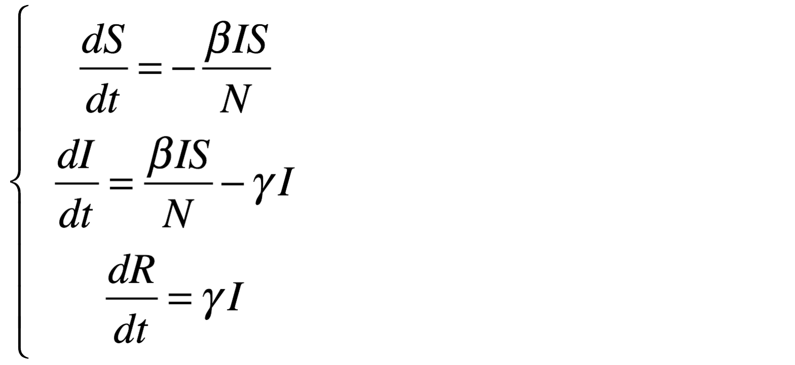
Given an initial condition (initial values) at time t=0, such as

• S = 499
• I = 1
• R = 0
• beta = 0.4
• gamma = 0.1
• h = 0.1

one can obtain the evolution of the evolution of S, I and R over time, by integrating the ODE system using a numerical scheme.

Why and when can we use ODE in agent-based models?

ODE models are often used when a system can be considered at a macro (population) level, i.e when the individual variability as little influence on dynamics at the aggregated level.

It is relevant to use ODE in agent-based models in several cases:

• Large scale agent-based models require many resources to run and a very large computation time. For example, if we want to implement a model describing the worldwide epidemic spread and the impact of air traffic on it, we cannot simulate the 7 billion people. Instead we can represent only cities with airports and airplanes as agents. In this case, cities are entities are represented by a compartment, on which a SIR class epidemiological model can be run, using an ODE system. Such a model combines some advantages of agent-based models (detailed description of the disease spread from one city to another with the plane agents) and mathematical modeling (good description of an epidemiological dynamics at a city level, using fewer resources and less computation time).

• Some processes may be easier to manipulate at the aggregated level, for several reasons: 1) a global description of a system may turn sometimes more informative than a detailed one, 2) a detailed description may require to fit too many parameters for which there is no sufficient data, in that case it is easier to fit a global model with less parameters, and 3) when one wants to keep a low number of parameters, in order to avoid overfitting or to optimize Akaike Information Criterion.

• Some systems are better described with a continuous dynamics than with a discrete one. This is the case for many physical or biological systems (physics laws such as gravity or water dynamics, biological processes such as respiration or cell growth). Coupling ABM and ODE model allow considering individual/discrete processes along with continuous processes.

• Some models already exist in an ODE version, and could be coupled to another model in Gama without having to rewrite an Agent-Based version of the model.

Use of ODE in a GAML model

A stereotypical use of ODE in a GAMA agent-based model is to describe species where some agents attribute evolution is described using an ODE system.

As a consequence, the GAML language has been increased by two main concepts (as two statements):

• equations can be written with the equation statement. An equation block is composed of a set of diff statement describing the evolution of species attributes.
• an equation can be numerically integrated using the solve statement

Additionnally, Gama provides an intuitive, flexible and natural framework to build ODE models, since an ODE system may be split among several entities. For example, if there are three species (resp. agent) involved in a common dynamics, it is possible to declare each equation inside the corresponding species (resp. agent) definition. An example is shown below.

Defining and solving an ODE system

Defining an ODE system with equation

Defining a new ODE system needs to define a new equation block in a species. As an example, the following eqSI system describes the evolution of a population with 2 compartments (S and I) and the flow from S to I compartments:

species userSI {
    float t ;
    float I ; 
    float S ; 
    int N ;
    float beta<-0.4 ;
    float h ;
	
    equation eqSI {
	diff(S,t) = -beta * S * I / N ;
	diff(I,t) = beta * S * I / N ;
    }
}			

This equation has to be defined in a species with t, S and I attributes. beta (and other similar parameters) can be defined either in the specific species (if it is specific to each agent) or in the global if it is a constant.

Note: it is mandatory to declare a differenciation variable (here t) as an attribute in the species. It is automatically updated using the solve statement and contains the time elapsed in the equation integration.

solve an ODE system

Once the equation or system of equations has been defined, it is necessary to execute a solve statement inside a reflex in order to numerically integrate the ODE system. The reflex is executed at each cycle, and the values of the attributes used in the equations (S and I in the previous example) are updated with the values obtained by integrating the system between the start time end and end time of the current cycle.

reflex solving {
    solve eqSI method: #rk4 step_size: h;
}

Several numerical schemes are available to solve the ODE system. More details about the numerical schemes and the solve syntax are provided below.

Alternative way to define an ODE system

Split a system into several agents

An equation system can be split into several species and each part of the system are synchronized using the simultaneously facet of equation. The system split into several agents can be integrated using a single call to the solve statement. Notice that all the equation definition must have the same name.

For example, the SI system presented above can be defined in two different species S_agt (containing the equation defining the evolution of the S value) and I_agt (containing the equation defining the evolution of the I value). These two equations are linked using the simultaneously facet of the equation statement. This facet expects a set of agents. The integration is called only once in a simulation step, e.g. in the S_agt agent.

global {	
    int N <- 1000;
    float hRK4 <- 0.01;
}

species S_agt {
    float t ;		
    float Ssize ;
	
    equation evol simultaneously: [ I_agt ] {
	diff(Ssize, t) = (- sum(I_agt accumulate [each.beta * each.Isize]) * self.Ssize / N);
    }
	
    reflex solving {solve evol method: #rk4 step_size: hRK4 ;}	
}

species I_agt {
    float t ;
    float Isize ; // number of infected	
    float beta ;

    equation evol simultaneously: [ S_agt ] {
	diff(Isize, t) = (beta * first(S_agt).Ssize * Isize / N);
    }
}

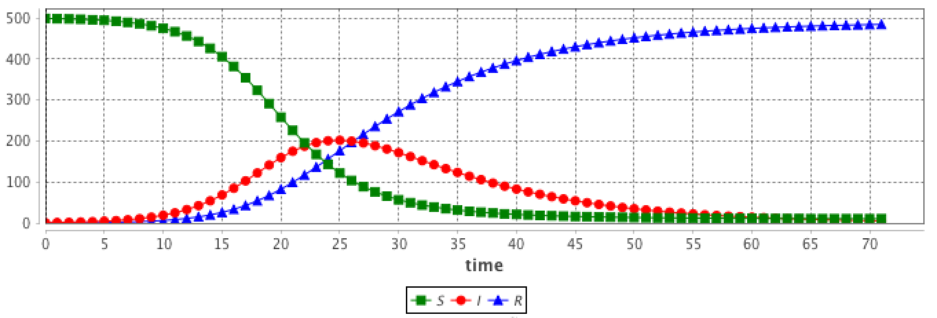
The interest is that the modeler can create several agents for each compartment, which different values. For example in the SI model, the modeler can choose to create 1 agent S_agt and 2 agents I_agt. The beta attribute will have different values in the two agents, in order to represent 2 different strains.

global {
    int number_S <- 495 ; // The number of susceptible
    int number_I <- 5   ; // The number of infected
    int nb_I <- 2;
    float gbeta  <- 0.3  ; // The parameter Beta
	
    int N <- number_S + nb_I * number_I ;
    float hRK4 <- 0.1 ;

    init {
	create S_agt {
	    Ssize <- float(number_S) ;
	}
	create I_agt number: nb_I {
	    Isize <- float(number_I) ;
	    self.beta <- myself.gbeta + rnd(0.5) ;
	}
    }
}

The results are computed using the RK4 (Runge-Kutta 4) method with:

• number_S = 495
• number_I = 5
• nb_I = 2
• gbeta = 0.3
• hKR4 = 0.1

Important note: the solve statement must be called once and only once per cycle. In this example, is it executed in the 'solving' reflex of the only S_agt agent. There is no 'solving' reflex in the I_agt agents: since the equations definitions blocks are connected through the simultaneously facet, there equation blocks will be integrated by the S_agt agent. Note also that if they were several S_agt agents, with the same definition of the 'solving' reflex, the solve statement would be executed several times, which could result in wrong results. To ensure that it is called only once, the 'solving' reflex should be rewritten. For example, it is possible to write this:

    reflex solving when: (int(self)=0) {solve evol method: #rk4 step_size: hRK4 ;}	

More details

Details about the solve statement

The solve statement can have a huge set of facets (see this page for more details). The basic use of the solve statement requires only the equation identifier. By default, the integration method is Runge-Kutta 4 with a fixed integration step of 0.005*step, which means that each simulation step (cycle) is divided into 200 smaller integration steps that are used to simulate a continuous evolution of the system.

For fixed integration step numerical schemes such as Runge-Kutta 4, the length of the integration step is defined in the step_size facet. Increasing the integration step results in faster computation at the cost of accuracy.

Integration method with the method facet

Several integration methods can be used in the method facet. GAMA relies on the Apache Commons Math library to provide numerical schemes; it thus provides access to the various solvers integrated into the library. The list of all the solver is detailed in this page, section 15.4 Available integrators. The GAML constants associated with each of them (to use in the method statement) are: )

• Fixed Step Integrators
  • #Euler for Euler. It implements the Euler integration method, which is mainly used for academic illustration of numerical schemes. It should not be used outside of this purpose due to its lack of precision (a very small integration step is required for an acceptable precision).
  • #Midpoint for Midpoint
  • #rk4 for Runge-Kutta 4. It implements the Runge-Kutta 4 integration method. It provides a faster convergence than the Euler method, and thus does not require very small integration steps. However the user has to determine manually the ideal integration step. For that reason, it is recommended to try first an adaptative stepsize integrator such as the Dorman-Prince 5(4) integration method.
  • #Gill for Gill
  • #ThreeEighthes for 3/8
  • #Luther for Luther
• Adaptive Stepsize Integrators
  • #HighamHall54 for Higham and Hall
  • #DormandPrince54 for Dormand-Prince 5(4) It implements the Dorman-Prince 5(4) integration method. It is similar to the ode45in Matlab. This method is based on the Runge-Kutta solvers family. It evaluates the error between the numerical solution and the analytic solution, and adapt the integration step in order to minimize it. It is recommended to try this method first, even it may not the best one in case of stiff problems.
  • #dp853 for Dormand-Prince 8(5,3).
  • #GraggBulirschStoer for Gragg-Bulirsch-Stoer
  • #AdamsBashforth for Adams-Bashforth
  • #AdamsMoulton for Adams-Moulton

Integration steps

The length of the integration step has a huge impact on precision: a smaller integration step means more evaluation points, which results in a better precision but a longer computation time. In order to improve the precision of the integration or its speed, the integration step can be set using the step_size facet for fixed steps methods.

• step_size (float): integration step, use with most fixed steps integrator methods (default value: 0.005*step)

Adaptative stepsize integrators (e.g. #DormandPrince54) automatically determine and set the integration step according to a given error tolerance. Some of them also use different integration steps all over the computation, since parts of the solution that are stable enough do not require a very small integration step, while parts with high variations need more precision. Such integrators require thus more information, through the following mandatory facets:

• min_step, max_step (float): these 2 values define the range of variation for the integration step. As an example, we can use: min_step:0.01 max_step:0.1.
• scalAbsoluteTolerance and scalRelativeTolerance (float): they defined the allowed absolute (resp. relative) error. As an example, we can use: scalAbsoluteTolerance:0.0001 scalRelativeTolerance:0.0001.

Synchronization between simulation and integration

The simulation and the integration are synchronized: if one simulation step represents 1 second, then one call of the solve statement will integrate over 1s in the ODE system. This means that the step attribute of the global has an impact on the integration. See below to observe this influence.

It is thus important to specify the unit of the parameters used in the ODE system (in particular relatively to time).

It is also important to notice that the integration step step_size will only control the precision of the integration. If step (of the global) is 1#s, then after 1 call of solve, 1#s has flowed in the equation system. If step_size is set to 1#s or to 0.01#s will not impact this fact. The only difference is that in the latter case, the solver made 100x more computations than in the former one (increasing the precision of the final result).

Additional facets

Here are additional facets that be added to the solve statement:

• t0 (float): the first bound of the integration interval (default value: cycle*step, the time at the beginning of the current cycle.)
• tf (float): the second bound of the integration interval. Can be smaller than t0 for a backward integration (default value: cycle*step, the time at the beginning of the current cycle.)

This might be useful more model coupling, when the sytem to integrate is not linked to the time evolution of the main simulation.

Intermediate results

In one simulation step, if the statement solve is called one time, several integration steps will be done internally. Intermediate computation results can be accessed using the notation: var[] that returns the list of intermediate values of the variable var involved in a differential equation. As an example, with a SIR equation:

species agent_with_SIR_dynamic {
    int N <- 1500 ;
    int iInit <- 1;		
    float t;  
    float S <- N - float(iInit); 	      
    float I <- float(iInit); 
    float R <- 0.0; 
	
    float alpha <- 0.2 min: 0.0 max: 1.0;
    float beta <- 0.8 min: 0.0 max: 1.0;
    float h <- 0.01;
   
    equation SIR{ 
	diff(S,t) = (- beta * S * I / N);
	diff(I,t) = (beta * S * I / N) - (alpha * I);
	diff(R,t) = (alpha * I);
    }
  
    reflex solving {
        solve SIR method: #rk4 step_size: h ;
    	
    	write S[];
      	write I[];
      	write R[];
    	write t[];
    }  
}

We can use S[], I[], R[] and t[] to access the list of intermediate variables of these 4 variables. SinceS[] is a list the first element can be accessed with S[][0].

Note that the current value of a variable, i.e. S, equals to the last value of the list S[]: S = last(S[]).

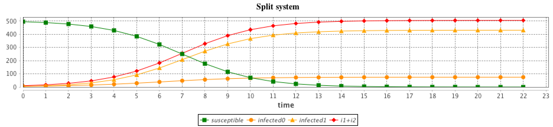
Accessing the intermediate values can be useful to provide smooth continuous charts. A way to do so is to provide the display with the full list of integration times and values, such as:

experiment continuous_display type: gui {
	output {	
		display display_charts axes: false{
			chart 'SIR' type: series x_serie: first(agent_with_SIR_dynamic).t[] y_range: {0,1000} background: #white {
				data "S" value: first(agent_with_SIR_dynamic).S[] color: #green marker: false;
				data "I" value: first(agent_with_SIR_dynamic).I[] color: #red marker: false;
				data "R" value: first(agent_with_SIR_dynamic).R[] color: #blue marker: false;
			}
		}
	}
}

The following picture illustrates the result: the top subfigure shows the dynamics with discrete visualization and the bottom one the continuous curves.

Example of the influence of the integration step

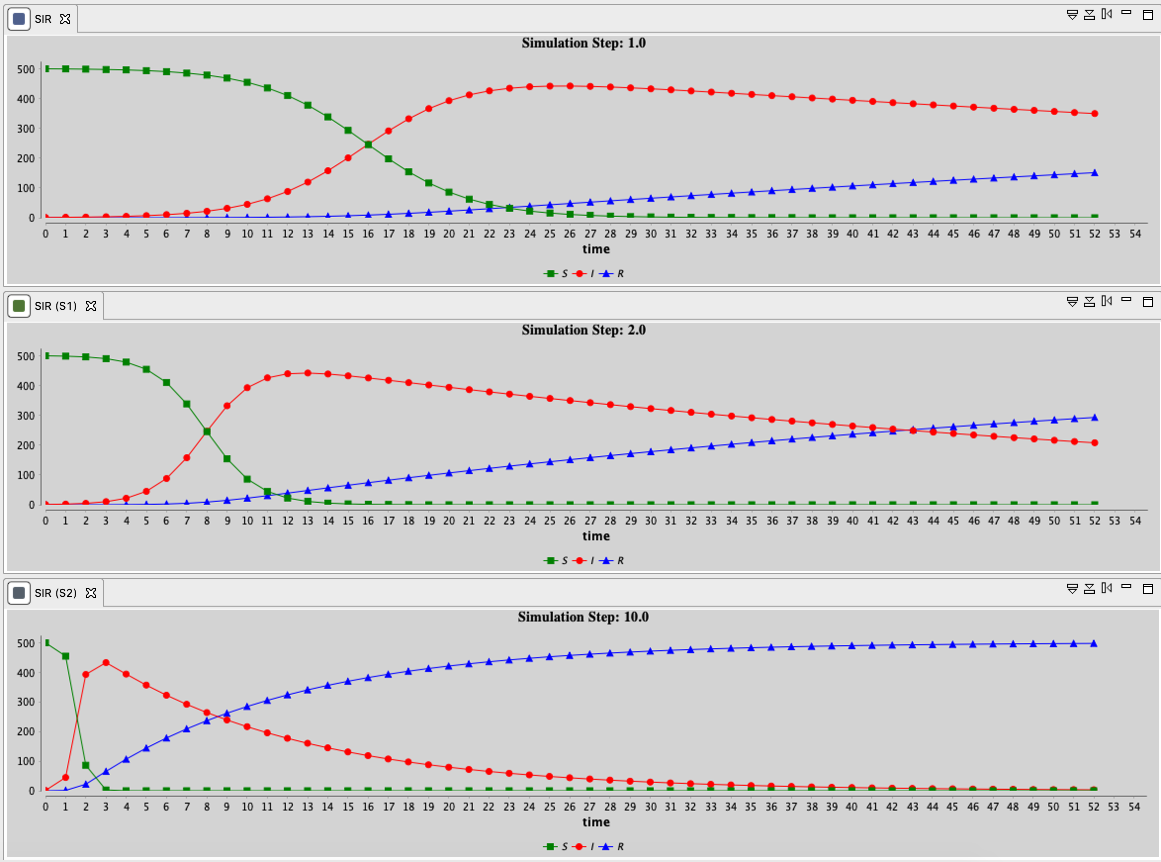
The step (of the global) and step_size (of solve) facets may have a huge influence on the results. step_size only has an impact on the result accuracy. The step facet changes the cycle duration and so the time scale and results in curves being horizontally scales.

In the following image, the stepfacet has been change from 1.0 (first simulation) to 2.0 (second simulation). The dynamics are exactly the same, but they are viewed at different time scales.

The following image illustrates this impact, by calling (with 3 different values of step):

When changing this facet, be sure that the time scale of the ODE system remains consistent with the one of the other agents.